【Rで統計】順序ロジスティック回帰分析

回帰分析をする際、

目的変数が Yes or No などの２つだと、通常のロジスティック回帰を行うが、

これが、例えば Not, Low, Intermediate, or High のように、

３つ以上の場合は、順序ロジスティック回帰を使う。

順序ロジスティック回帰をRで行う方法

"ordinal" パッケージをインストール

install.packages("ordinal")
library("ordinal")

"clm" を使う

方法は、

clm(目的変数 ~ 説明変数1 + 説明変数2 ..., データ = データ名)

のような形で使用する。

• 目的変数: 疾患のステージ "Stage"
  • Stage 0: "0"
  • Stage 1: "1"
  • Stage 2: "2"
  • Stage 3: "3"
  • Stage 4: "4"

• 説明変数1: 遺伝子多型 "Genotype"
  • CC: ダミー変数 "0"
  • CT: ダミー変数 "1"
  • TT: ダミー変数 "2"
• 説明変数2: 年齢 "Age"
• 説明変数3: 性別 "Sex"

• データ: "myData"

model <- clm(Stage ~ Genotype + Age + Sex, data = myData)

サマリーを抽出。

res1 <- summary(model)
res1

output
> model <- clm(as.factor(LATE_Stage_2) ~ rs5848 + Age + Female, data=Data_G)
> res1 <- summary(model)
> res1

formula: Stage ~ Genotype + Age + Sex
data: myData

Coefficients:
            Estimate Std. Error z value Pr(>|z|)
GenotypeTC   0.53720    0.36580   1.469 0.141948
GenotypeTT   1.69885    0.50303   3.377 0.000732 ***
Age          0.08865    0.02414   3.672 0.000240 ***
Sex          0.21037    0.39985   0.526 0.598808
---
Signif. codes: 0 ‘***’ 0.001 ‘**’ 0.01 ‘*’ 0.05 ‘.’ 0.1 ‘ ’ 1

Threshold coefficients:
   Estimate Std. Error z value
0|1  8.712       1.956   4.454
1|2  9.548       1.976   4.832
2|3  10.382      2.004   5.182
3|4  10.930      2.025   5.398

上記の結果、P value "Pr(>|Z|)" は、TT で 0.000732。

reference は CC にしているので、この場合、

「TT を持つ人は CC を持つ人よりも疾患のステージが上がる」」

と言える。

また、年齢 "Age" も有意差がついているので、

「さらに、年齢が高いほど疾患ステージが高い」

と言える。

「オッズ比」と「95％CI」も出してみる

予め

round

関数で、表示する小数点以下レベルを決めておいた方が良い。

私は、

• オッズ比 "OR" は 小数点2桁まで
• 95％CI "ORlow", "ORhigh" は小数点2桁まで
• 標準偏回帰係数 "β" は小数点3桁まで

算出したいので、下記のように記述。

OR <- round(exp(coe[,1]), 2)
ORlow <- round(exp(coe[,1]-1.96*coe[,2]), 2)
ORhigh <- round(exp(coe[,1]+1.96*coe[,2]), 2)
res2 <- round(cbind(coe,OR,ORlow,ORhigh), 3)

res2

output
> OR <- round(exp(coe[,1]), 2)
> ORlow <- round(exp(coe[,1]-1.96*coe[,2]), 2)
> ORhigh <- round(exp(coe[,1]+1.96*coe[,2]),2)
> res2 <- round(cbind(coe,OR,ORlow,ORhigh), 3)
>
> res2

          Estimate Std. Error z value Pr(>|z|)       OR   ORlow     ORhigh
0|1          8.712      1.956   4.454    0.000  6076.87  131.38  281077.45
1|2          9.548      1.976   4.832    0.000 14016.31  291.39  674213.15
2|3         10.382      2.004   5.182    0.000 32276.75  635.97 1638110.86
3|4         10.930      2.025   5.398    0.000 55825.90 1055.25 2953353.75
Genotype TC  0.537      0.366   1.469    0.142     1.71    0.84       3.50
Genotype TT  1.699      0.503   3.377    0.001     5.47    2.04      14.66
Age          0.089      0.024   3.672    0.000     1.09    1.04       1.15
Sex          0.210      0.400   0.526    0.599     1.23    0.56       2.70

上記から、"TT" は全てのステージにおいて影響を与えていると言える。

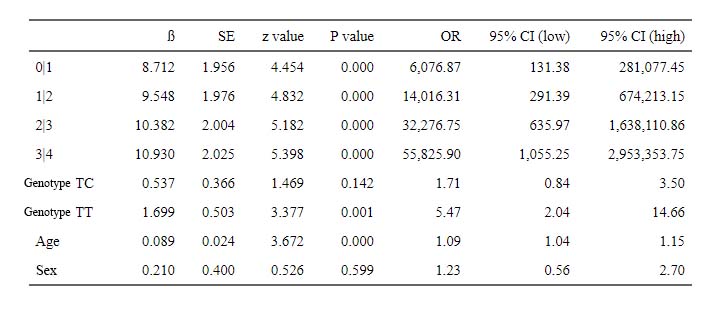
表として出力

表として出力する。

まずは、上記のデータを

as.data.frame

でデータフレームに変換し、

表のヘッダーの名前を

rename

で、それぞれわかりやすい表示に変更し、

必要な項目のみ

select

で選出する。

res3 <- res2 %>%
as.data.frame(row.names = row.names(model)) %>%
mutate(" " = rownames(res2)) %>%
rename("β" = Estimate, "P value" = "Pr(>|z|)", SE = "Std. Error", "95% CI (low)" = ORlow, "95% CI (high)" = ORhigh) %>%
select(" ", "β", "SE","z value", "P value", "OR", "95% CI (low)", "95% CI (high)")

そして、

flextable

で表として出力。

res3 %>%
flextable::regulartable() %>%
flextable::theme_booktabs() %>%
flextable::font(fontname = "serif", part = "all") %>%
flextable::autofit()

出力結果 ▼